Tutorial: Collisionless Shocks

This tutorial provides some tips for getting started with collisionless shock simulations using Runko.

Simulation scripts and analysis files for shock simulations are found in

/runko/projects/pic-shocks

The pic-shocks project simulates a scenario where plasma travels in a tube-like structure in the \(-x\) direction, meets the end of the tube and reflects back towards the \(+x\) direction. As a result, there are two populations of plasma passing through each other. The populations interact with each other via the electromagnetic fields and form a collisionless shock.

The example setup simulates a relativistic, magnetized, perpendicular shock in an electron-positron pair plasma. Such shocks are prone to the synchrotron maser instability. More details are available, e.g., in Plotnikov & Sironi 2019.

Running the Simulation

Simulations as well as analytical procedures are run via command line. The syntax for running the simulation is

mpirun -n [number of cores] python3 pic.py --conf file.ini

The above command executes file pic.py using [number of cores] MPI ranks and configuration parameters set in file.ini. The amount of MPI ranks depends on your machine.

Example: Running a simulation with 4 cores using the configuration file 2dsig3.ini:

mpirun -n 4 python3 pic.py --conf 2dsig3.ini

Configuration Parameters

Grid and Dimensions

Simulations are available in all three dimensions and you can set the size of the grid based on your needs. The following configuration parameters are found and can be edited in the .ini files.

Simulation framework:

• [grid]

  • Nx, Ny, Nx : Number of tiles in corresponding directions

  • NxMesh, NyMesh, NzMesh : Number of partitions each tile is divided into in each corresponding direction; internal grid.

  • c_omp : Simulation skin depth resolution

Complete grid size in each dimension is determined as Ni*NiMesh. One plasma skin depth (in the upstream) equals \(\texttt{c_omp} \times \texttt{cells}\).

Relevant parameters to get the simulation running:

• [io]

  • outdir, prefix, postfix : Output directory name

  • interval : Simulation output frequency for analysis in units of laps

The output directory can be easily named by defining outdir: "auto" and setting, e.g., prefix: "shock_" and postfix: "_try1"; this will automatically create a folder shock_XXX_try1, where XXX is replaced with the simulation parameters.

• [simulation]

  • Nt : Maximum simulation time in units of laps

  • npasses : Number of current filters

  • mpi_track : Caterpillar cycle length

• [problem]

  • delgam : Upstream plasma temperature in units of \(\frac{kT}{m_e c^2}\)

  • bpar, bplan, bperp : Magnetic fields in \(x\), \(y\) and \(z\) directions accordingly.

  • sigma : Plasma magnetization parameter, \(\; \sigma = \frac{B^2}{4\pi n_e \gamma m_e c^2}\)

  • gamma : Upstream bulk flow speed in units of

    • Lorentz factor \(\quad \Gamma = \left(1 - \frac{v^2}{c^2} \right)^{-\frac{1}{2}}, \quad\) for \(\gamma > 1\)

    • 3-velocity \(\quad \beta = \frac{v}{c}, \quad\) for \(\gamma < 1\)

• [particles]

  • Npecies : Number of particle species

  • ppc : Particles per cell per species

  • n_test_prtcls : Number of test particles

Analysis Tools

Scripts

The pic-shocks folder includes some python scripts for plotting the simulation data.

• plot_upstream_ene.py plots the Poynting flux of the synchrotron maser as well as the components of electromagnetic fields in a region of upstream plasma ahead of the shock.

• plot_jump_conds.py calculates the shock jump conditions and plots them; plots the \(x\) location and velocity of the shock as well as the downstream to upstream plasma density ratio as functions of simulation time steps.

• plot_dens.py plots the plasma density as a mountain plot.

• plot_win_2d_shock.py visualizes the shock; plots plasma densities, velocities and components of electric and magnetic fields and electric currents into individual panels.

Usage

All of the scripts above use syntax

python3 script.py --conf file.ini

Except in case of plot_win_2d_shock.py:

python3 plot_win_2d_shock.py --conf file.ini --lap [lap number]

The number after --lap specifies the simulation lap you want to view. If you want to plot all of the laps of a complete run, you can run

./scripts.sh

in the pic-shocks folder.

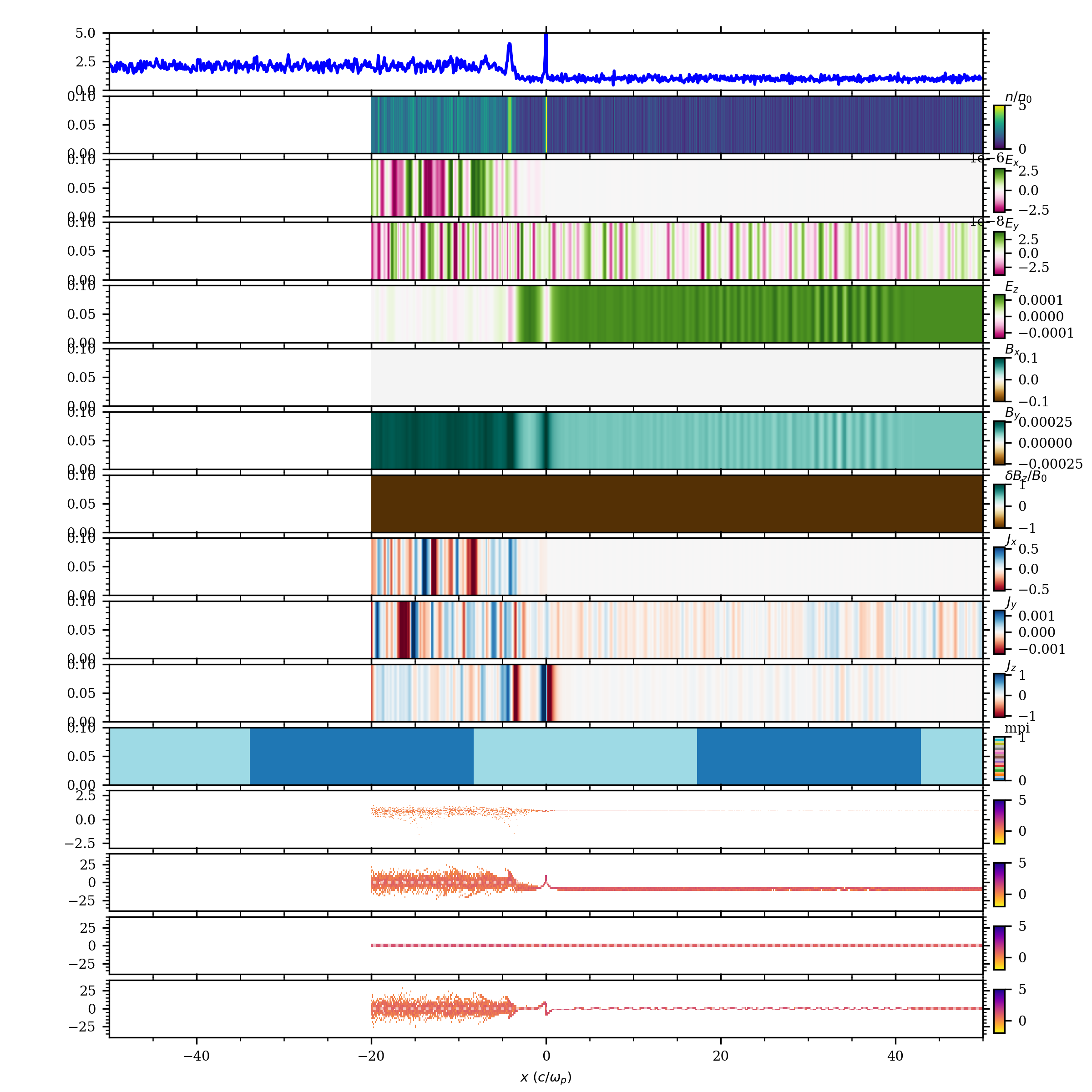
Example: The output of plot_win_2d_shock should look something like this:

Note

The above plot is from a short 1D shock simulation (with \(\gamma = 10\) and \(\sigma = 3\)) using 2 cores. Depending on the dimensions and other parameters of your simulation the output might look slightly different.

The script plots the values in panels as functions of skin depth, \(\frac{c}{\omega_p}\) (scale at the bottom of the figure). Point \(x = 0\), which follows the shock front, divides the plasma into downstream (negative \(x\)) and upstream (positive \(x\)) sections.

The top two panels show plasma density. If a shock has succesfully formed, you should be able to see a jump in the downstream to upstream density affected by the shock: \(\frac{n_d}{n_u} \approx 1 \rightarrow 2\)

Other panels include (top to bottom) \(x\), \(y\) and \(z\) components of the electric field, magnetic field and electric currents. Panel just beneath \(J_z\) marks the MPI rank division. The bottom four panels visualize the total velocity \(\log_{10}(\gamma)\) and the individual four-velocity components \(\beta_x \gamma\), \(\; \beta_y \gamma\), and \(\; \beta_z \gamma\).